Load forecasting at the secondary substation level
At Elvia, Norway’s biggest distribution operators system, we had the chance to host our first Data Science Summer Camp. Four students (Anne Willkommen Eiken, Chanjei Vasanthan, Jonas Nagell Borgersen and Kaia Idun Bonnet) were gathered from the 15th of June to the 15th of August to work as a group on one topic, within the limits authorized by the health authorities. Gard Støe, at the origin of this initiative, and myself. This blog entry presents the results of these 8 weeks of work
Table of content:
Use-Case
The students decided to deepen the use-case entitled load forecasting at the secondary substation level. Elvia AS has roughly 25’000 secondary substations in its grid. One substation contains one or more transformers (TFs) that brings voltage down from 11/22 kV to 240/400V 1. From these transformers, the electricity goes directly to the end users. As depicted in Figure 1, the electricity (or load) consumption of the end users connected to each TF will be the main driver of the electricity load that transits through the transformer.
This load is what we are interested in forecasting. Several potential short- and long-term use cases can be interested in such forecast :
- preventing overload of the transformer
- steering batteries installed on low-voltage grid
- etc…
In our case, we were interested in showing the technical feasibility of forecasting load at almost the finest granularity of an electricity grid network. By experience, we know that forecasting country level load is easier than forecasting end user level load, and therefore wanted to tackle the hardest use case for a DSO.

Forecasting the load of one TF is of course interesting. But we identified very early the need to address all TF, not just one. As a consequence, we understood very early that having 25’000 models in production was not desirable. In addition, as shown in Figure 1 with tr1 and tr2, substations with similar type of end user present similar load patterns. With both this in mind, the students investigated a method to reduce the amount of models using these load similarities.
Clustering similar substations based on either existing labels or purely based on data was then added before forecasting so that we need K models (where K is the number of models) instead of N models (where N is the number of substations). A schematic of the workflow we had set up for this summer camp can be seen in Figure 2 : pre-processing, clustering and forecasting.

Pre-processing
Very briefly described the pre-processing done to each timeserie tr(t). First we removed negative-load (?!) and zero-load values. The data was then z-transform : \(z_{tr}(t) = \frac{tr(t) - \mu_{tr}}{\sigma_{tr}}\) where $\mu_{tr}$ and $\sigma_{tr}$ are respectively the mean and the standard deviation measured during the whole historical period. Finally, we created for each z-transformed substation load a weekly average by averaging every instance of time and day of the week in the historical period. For example, the first point of this weekly average corresponds to Monday at 01:00: this point was obtained by averaging all Mondays at 01:00 found in the historical period.
In addition to this data pre-processing, we assigned a sector-label to each substation. This substation sector-label is based on the sector (type) of the end-users connected to it that has the highest annual consumption. Let’s look at one example:
| End-user type | Amount | Annual consumption (kWh) |
|---|---|---|
| Industry | 2 | 392762 |
| Other | 1 | 1230 |
| Household | 6 | 47163 |
In the example of Table 1, the substation has 9 end-users connected to it with Household being the type with most end-users. But we also see that the annual consumption for the label Industry is higher than for Household, and therefore this substation will get the sector-label Industry attached to it.
With this method, we obtained 22 different sector-label substation in the whole dataset. To make the analysis easier, we limited our study to the three sector-labels with most substations: household (4134), cabin (379) and industry (229).
Clustering
Two main clustering approaches were used/tested:
- label-driven clustering: each substation is clustered solely based on the label assigned (based on end user category, see previous chapter)
- data-driven clustering: each substation is clustered solely based on the consumption pattern
Both methods allow to reduce the input data space from N to K and to create clusters of similar consumption patterns. Assessing clusters is dependant on how one uses these clusters. Depending on the use, we might be interested more in one of these cluster properties: compactness, differentiability, substantiality and stability 2. In our case, we are interested in validating the clusters in conjunction with the forecasts results, more about this in the last part of the blog post.
A bit more details about assumptions underlying label-driven and data-driven clustering.
Label-driven clustering
This is the easiest to understand: each substation is assigned to its cluster based on the label assigned during the pre-processing step. Because of how the assignment of the label was done, we expect that the consumption pattern will be similar within each cluster.
The advantage of this method is that it is easy to implement, computationally inexpensive, and you don’t have to define a temporal period where you define a consumption pattern (daily, weekly, monthly, yearly, etc…) prior to the clustering.
But the main disadvantage is that the sector-label for each substation is derived from sector-labels for end-users which are manually entered in the database and there are prone to errors or changes (the famous kingdom of dirty data). Concrete example seen: a nursery that is registered as household. This could potentially mislabel substation, and therefore make the clusters less homogeneous. In addition, this method limits the number of cluster K to the existing number of sector-labels.

Data-driven clustering
In the purely data-driven cluster, the algorithm (K-Means, K-Shape, Hierarchical) looks for similarities in the data to decide about the members of the clusters. I’ll let the reader Google the name of these algorithms and read more about the theory about how we obtain clusters that have smallest intra-cluster distance and the largest inter-cluster distance.
I would emphasize more about the choices made during this summer camp. First, we decided to standardize the z-transformed load timeseries by generating a weekly average of the whole historical period accessible for each TF. We then obtained a 168 data points per TF, the first point of this new representation of the data being for example the average of all Mondays at 01:00 that exist in the whole historical period.
The choice of using week instead of day or month is rather related to the consumption patterns in households, industries and even more cabins.

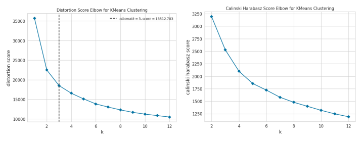
When clustering the data using K=3 and the K-means algorithm, the cluster generated are very similar to the clusters to the one obtained in the label-driven clusters (Figure 4). Interestingly, we see that the optimal number of cluster based on the elbow method with the distortion metric is 3 (Figure 5, left), but we also see that the “elbow” is very smooth and that changing metric (Figure 5, right) makes the optimal number cluster not possible to detected. .
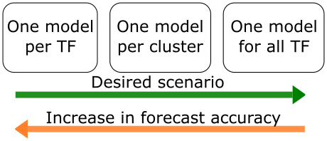
The advantage of these data-driven methods are that the number of cluster K is a hyper-parameter that the user can set prior to running the algorithm. This is essential to study more in detail how reducing the number of forecasting models by means of clustering influences the forecasting accuracy. Very early, the tradeoff (Figure 6) between number of models and accuracy was identified by thinking about the extreme cases:
K=N: one model per substation, too many models but best forecasting accuracyK=1: one model for all substations, ideal scenario in term of number of models, but loss in forecasting accuracy
Forecasting
The ingredients necessary for training a forecasting model were discussed early in the summer camp:
- what models to test
- what features to investigate
- what cases should we run through
The problem we are trying to solve here is a regression problem, and as Bishop defines in his seminal book:
The goal of regression is to predict the value of one or more continuous target variables t given the value of a D-dimensional vector x of input variables (or features). Given a training data set comprising N observations {xn}, where n = 1, . . . , N, together with corresponding target values {tn}, the goal is to predict the value of t for a new value of x. In the simplest approach, this can be done by directly constructing an appropriate function y(x) whose values for new inputs x constitute the predictions for the corresponding values of t.
The function y is an approximation (model) of the process that generates the target t.
Models
The recommendation made to the students were as follows: first test some models using the default hyperparameters and the same set of features (what I call light test). Then based these early results, choose the ones that seem to be responding well, and study these 3-4 models of interest more in depth.
We deliberately didn’t test the classical TS forecasting models like ARIMA, but focused on ML models. The students were active and looked at successful Kaggle models, used Google a lot and ended up looking and light testing the following models: Random Forest Regressor, Gradient Boosting Regressor, Support Vector Machine, Ridge regression, Lasso regression, Facebook Prophet, Nbeats, Sequential, CatBoost Regressor and LightGBM Regressor.
Out of this mountain of models, four models were selected for a deeper look:
- Random Forest Regressor
- Gradient Boosting Regressor
- CatBoost Regressor
- Facebook Prophet
Features
As one can see in the tr1 and tr2 of Figure 1, Norwegian consumption variability is negatively correlated with the outside temperature. We also expect the consumption to be variable in relation the hour of the day, the day of the week and the local holidays. More interesting, we saw that load same hour some days back is a good predictor for future load. After some iterations, we settled on using the load 7 days, 4 days and 3 days in the past as features. Finally, we added weekly average of the historical data (sort of normal curve). In fine, these are the features used:
- five continuous features
- Load for 7, 4 og 3-days in the past
- Weekly average of the historical load
- Temperature (historical forecasts)
- four categorical features:
- Hour ∈ [0, 23]
- Day of the week ∈ [0, 6]
- Month ∈ [1, 12]
- Holidays ∈ [True, False]
Cases
Three cases were implemented to test the set of features and models presented above:
- Case 1: predicting individual substations with one model per substation
- Case 2: predicting individual substations with one model per cluster
- Case 3: predicting individual substations with one model for all substations
By studying these three cases, we ought to show the degradation of the accuracy metric as we hypothesized that the accuracy metric (we choose MAPE, mean percentage absolute error) is going to degrade as follows:
\[MAPE_{case1} < MAPE_{case2} < MAPE_{case3}\]where the MAPE (%) is expressed as:
\[MAPE = 100 * \frac{\sum_{t=1}^{67}\widetilde{tr}(t)-tr(t)}{\sum_{t=1}^{67} tr(t)}\]where $\widetilde{tr}(t)$ is the model prediction at time t and $tr_t$ is the true value at time $t$.
Results
All the models were trained using historical data spanning the period from 1 June 2018 to 31 January 2020. Cross-validation was done for the four models to select the best set of hyperparameters. The models were trained using historical weather forecasts from Thredds API nicely pre-processed and accessible through an internally developed API. We then tested the models using the load/features from 1st Feb 2020 to 13th March 2020.
We decided to focus on short-horizon forecast (couple of days ahead). The Norwegian meteorological institute API provides freely accessible hourly weather forecast 67 hours in the future. Therefore, the models were tested for 15 forecast horizons (67 hours), as 67 hours x 15 covers the test period.
To make it easy to read, we chose two substations of each sector studied (household, cabin and industry).
Case 1. Predicting using one model per NS
In this case, we have optimized each model’s hyperparameters by using cross-validation method. We interestingly observed that default hyperparameters for CatBoost were already very close to the optimal set of hyperparameters obtained at the end of the lengthy CV run.


In Figure 7, we can visually assess the performance of the four models when predicting one forecast horizon (67 hours) for six individual substations. A general impression, confirmed by the quantitative assessment in Table 2., is that the three tree-based models perform rather similarly, succeeding in predicting the household and industry substations, but having some problems with the cabin ones. Prophet prediction seems to smoother but more inaccurate than the tree-based models. If we average the 67 points of one forecast horizon, and predict 15 forecast horizons (and take the mean and std of these 15 forecast horizons), we obtain the results in Table 2.
| House 1 | House 2 | Cabin 1 | Cabin 2 | Industry 1 | Industry 2 | |
|---|---|---|---|---|---|---|
| $\mu$ $\pm$ $\sigma$ | $\mu$ $\pm$ $\sigma$ | $\mu$ $\pm$ $\sigma$ | $\mu$ $\pm$ $\sigma$ | $\mu$ $\pm$ $\sigma$ | $\mu$ $\pm$ $\sigma$ | |
| Random Forest | 3.5 $\pm$ 0.42 | 5.3 $\pm$ 1.4 | 11.5 $\pm$ 6.8 | 10.1 $\pm$ 4.7 | 5.2 $\pm$ 1.6 | 6.4 $\pm$ 3.4 |
| Gradient Boosting regressor | 3.6 $\pm$ 0.48 | 6.2 $\pm$ 1.6 | 12.2 $\pm$ 7.9 | 11.2 $\pm$ 3.6 | 5.9 $\pm$ 1.9 | 6.2 $\pm$ 2.8 |
| CatBoost Regressor | 3.5 $\pm$ 0.33 | 6.2 $\pm$ 1.7 | 12.1 $\pm$ 8.0 | 10.6 $\pm$ 3.5 | 5.5 $\pm$ 1.7 | 5.9 $\pm$ 3.0 |
| Facebook Prophet | 4.6 $\pm$ 0.90 | 15.4 $\pm$ 5.0 | 10.9 $\pm$ 5.0 | 13.2 $\pm$ 6.2 | 7.4 $\pm$ 2.3 | 8.6 $\pm$ 2.7 |
There are several interesting results within Table 2:
- The metrics obtained for all three tree-based models are roughly similar, whereas Prophet is worse in 5 out of 6 cases. Without entering into details of Prophet, we generally didn’t see the potential of using this model for short-term load forecasting.
- The level of accuracy obtained for house and industry (~5%) is very promising, with feature load-7 being the feature with most importance with random forest. A deeper investigation at feature importance, for example looking at SHAP values, could be a possible follow-up.
- The level of accuracy obtained in cabin is roughly 2 times worse than house and industry. One possible explanation is that the set of features lack predictability for cabin electricity use. For example, load-7 is not a very good predictor as there is not an obvious weekly repetition of cabin use. Other features like snow level, precipitation (bad weather->less people going to cabins) and more detailed holidays (days before and after included) could be investigated to potentially make these cabin predictions better.
Case 2. Predicting using one model per cluster
Now comes the interesting bit: the number of clusters K varies (30, 20, 15 and 10) and the forecast is done using the model trained using all the members of each clusters together. For the case of clarity, we only report the results with one model, CatBoost regressor.
| House1 | House2 | Cabin1 | Cabin2 | Industry1 | Industry2 | |
|---|---|---|---|---|---|---|
| $\mu$ $\pm$ $\sigma$ (CS) | $\mu$ $\pm$ $\sigma$ (CS) | $\mu$ $\pm$ $\sigma$ (CS) | $\mu$ $\pm$ $\sigma$ (CS) | $\mu$ $\pm$ $\sigma$ (CS) | $\mu$ $\pm$ $\sigma$ (CS) | |
| K=10 | 4.3 $\pm$ 0.54 (80) | 6.3 $\pm$ 1.3 (906) | 10.4 $\pm$ 4.0 (486) | 10.1 $\pm$ 3.0 (486) | 6.2 $\pm$ 1.4 (131) | 8.3 $\pm$ 4.0 (65) |
| K=15 | 4.3 $\pm$ 0.60 (42) | 6.3 $\pm$ 1.4 (585) | 10.1 $\pm$ 3.6 (438) | 10.2 $\pm$ 2.7 (438) | 5.8 $\pm$ 1.6 (102) | 8.1 $\pm$ 4.0 (58) |
| K=20 | 4.0 $\pm$ 0.64 (18) | 6.6 $\pm$ 1.8 (376) | 10.9 $\pm$ 3.8 (354) | 10.7 $\pm$ 2.8 (354) | 6.0 $\pm$ 1.6 (98) | 7.7 $\pm$ 4.1 (22) |
| K=30 | 4.0 $\pm$ 0.64 (18) | 6.8 $\pm$ 1.6 (335) | 9.0 $\pm$ 4.9 (306) | 11.2 $\pm$ 3.3 (306) | 5.7 $\pm$ 1.6 (74) | 8.1 $\pm$ 4.2 (19) |
| K=5449 | 3.5 $\pm$ 0.33 (1) | 6.2 $\pm$ 1.8 (1) | 12.1 $\pm$ 8.0 (1) | 10.6 $\pm$ 3.5 (1) | 5.5 $\pm$ 1.7 (1) | 5.9 $\pm$ 3.0 (1) |
As we increase the number of clusters K, we rightly observed that the cluster size diminishes. We expect that the members of each clusters are closer to each other, and therefore expect that the generative process that we try to model are close enough that we can use one model without big loss of accuracy. It is very interesting to note that this is not always true in the experiment we ran. Out of 6 substations, only 2 (house 1 and industry 2) show a clear decrease in accuracy from few clusters (10) to one model per substation (5449). In addition, it is also interesting to note that substation with poor forecasting accuracy with one model per substation (cabin1 and cabin2) got better accuracy when clustering. Further work should be done to understand this. One possible explanation is that the amount of data used when training one model per substation (20 months) is too limited, ahd therefore combining similar substations within the same model allows learning more complex relationships between features and output.
Discussion
This was our first deep dive into forecasting problems at Elvia. We have now an idea about the possibilities, the possible accuracy of the short-horizon forecasts we could provide to our domain experts sitting at the control centre. The students have done a tremendous job into setting up what will be our reference pipeline to quickly customized future forecasting problems. The normal continuation of this project would be to optimise the number of cluster and the accuracy of the models at the same time to find a sweet spot where both K and accuracy are optimized simultaneously (Figure 8).

When it comes to Case 3 (one model for all substation), we were confronted to technical limitations of the technology stack (Azure Blob + Jupyter Notebook in AzureML) used during the camp. When number of rows in the feature matrix is over hundred of millions, then focus on speed of execution is mandatory. Apache Spark seems to be a good candidate for solving this, but I am sure many others exists as well.
One step further, the problem of learning in deep learning (DL) is cast as a search or optimization problem to navigate the space of possible sets of weights the model may use in order to make good enough predictions. This optimization is coded in the loss function of the DL framework. So we might think that with an appropriate DL architecture and loss function, one could simplify the problem to one DL model. This idea is rather attractive, and further investigation of its potential implementation is being discussed together with the ML group in Tromsø.

Last but not least, I would like to thank the four students for their amazing contribution during these two months, where team work was reduced to discussion over the Internet and some very few (but intense and constructive) physical meetings over the whiteboard. Please contact with me by email or on LinkedIn